This preview is for read-only use. Code is inoperable.

Machine Learning Applications in the Earth Systems Sciences

In this module, you will build upon the knowledge from Machine Learning Foundations in the Earth Systems Sciences by executing tasks with code and interactive widgets. Expect to leave this module with a deeper understanding of data exploration, the iterative process of machine learning development, and critically judging machine learning model output.

Optimize a precipitation classification machine learning model

Previously, Sam and the research team made their first supervised machine learning classification model. This proof-of-concept model showed some skill, but the team ultimately decided to ask for help before proceeding any further. This is where you come in. Play the video below to learn more about how you will help Sam and the team refine their model and ultimately make a decision on whether the model is appropriate for the task.

Video opens in a new tab.

Transcript

What is a machine learning engineer?

Now that you know the process for developing a supervised machine learning model, you have a general idea of all the tasks that machine learning engineers are tasked with. From problem framing through model evaluation, machine learning engineers work with decision makers and data specialists to design and develop machine learning models. In addition to the machine learning skills you have learned so far, machine learning engineers have skills in Python programming, data science, statistics, and importantly, domain-specific knowledge.

---

Part 1: Problem Framing

Recall that the first step in developing a machine learning model is problem framing.

Click to enlarge

Sam and the team have already completed the problem framing step based on the task from their supervisor. Review their framing questions below.

Problem framing questions

Does a simpler solution exist?

 Predicting the type of precipitation during a winter weather event relies on many different co-varying variables, including differences in temperature and humidity between the surface and clouds and winds, to name a few. A simple conditional statement may not be the most effective tool.

Can machine learning requirements be met?

 Sam will use a weather forecasting model in combination with citizen scientist precipitation type reports during winter weather events. They will have thousands of data records to use in development.

Which scientific question should be answered?

 "Will the precipitation at a certain location and time be rain or snow?"

---

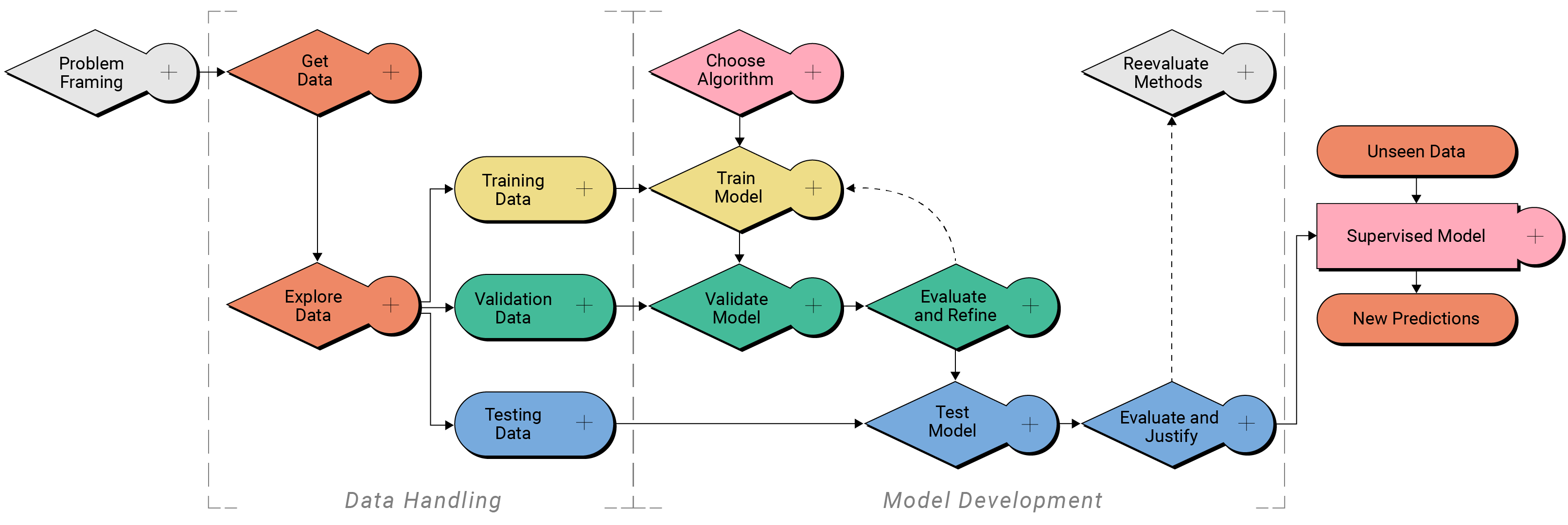
Part 2: Data Handling

Data handling is the multi-step process for preparing data for model development. During this phase, data are gathered, examined, and split into three groups for model development and evaluation.

Click to enlarge

Part 2a: Locate Data of Interest

Sam's team has already gathered the data to use in model development and shared it with you to review. They combined output from the atmospheric reanalysis model output with citizen science precipitation type reports from mPing (NOAA NSSL, University of Oklahoma) such that every precipitation report corresponds to a series of environmental variables at the same time and location. These data are open-access so they did not need to gain special permission for use.

They also want to make this new dataset available for other scientists and researchers (like you!) to use and build upon their progress, so they have made the data available to everyone following the FAIR data principles.

FAIR data principles

FAIR data principles ensure that data are Findable, Accessible, Interoperable, and Reusable by the scientific community. Following FAIR data principles helps ensure that research is transparent, reusable, and contributes to the peer-review process that keeps science reliable and open to improvement.

To clearly document the source and nature of the data, they have created the following metadata document. Review this information before starting the next step: exploring the data.

Metadata Document for Precipitation Type Classification Data

General Information

Dataset Name: Precipitation Type Classification Data

Description: Combination of atmospheric reanalysis model output and mPing precipitation reports.

Date Range:

Geographic Coverage: Continental United States

Data Frequency: Irregular, one record per mPing report

Last Updated: 02/02/2025

Data Structure

File Format: .parquet

Number of Records: 5000

Columns (features):

• TEMP_C_0_m: Air temperature (°C) at 0 meters above ground level.
• TEMP_C_1000_m: Air temperature (°C) at 1000 meters above ground level.
• TEMP_C_5000_m: Air temperature (°C) at 5000 meters above ground level.
• T_DEWPOINT_C_0_m: Dewpoint (°C) at 0 meters above ground level.
• T_DEWPOINT_C_1000_m: Dewpoint (°C) at 1000 meters above ground level.
• T_DEWPOINT_C_5000_m: Dewpoint (°C) at 5000 meters above ground level.
• PRES_Pa_0_m: Environmental pressure (Pa) at 0 meters above ground level.
• PRES_Pa_1000_m: Environmental pressure (Pa) at 1000 meters above ground level.
• PRES_Pa_5000_m: Environmental pressure (Pa) at 5000 meters above ground level.
• UGRD_m/s_0_m: U-component (west to east) of wind speed (m/s) at 0 meters above ground level.
• UGRD_m/s_1000_m: U-component (west to east) of wind speed (m/s) at 1000 meters above ground level.
• UGRD_m/s_5000_m: U-component (west to east) of wind speed (m/s) at 5000 meters above ground level.
• VGRD_m/s_0_m: V-component (south to north) of wind speed (m/s) at 0 meters above ground level.
• VGRD_m/s_1000_m: V-component (south to north) of wind speed (m/s) at 1000 meters above ground level.
• VGRD_m/s_5000_m: V-component (south to north) of wind speed (m/s) at 1000 meters above ground level.
• ptype: Precipitation type reported to mPing ("rain" or "snow")

Data Quality

Missing Data: There is no missing data in this dataset

Outlier Handling: No outlier handling was done

Data Provenance

Sources: Our research group provided the reanalysis mdoel output. Precipitation type reports are from mPing (NOAA NSSL, University of Oklahoma)

Part 2b: Explore Data

Now it's your turn to explore the data that the team has prepared. Before starting an analysis of any kind, it's important to familiarize yourself with the data before you use it. This way, you can identify any issues or limitations in the dataset before you start generating statistics or transforming the data. In this step, you will take a closer look at the input and target features with a few plots.

First, let's read the data into this workspace. To begin, we must import several Python packages, including all the tools for reading the data from the THREDDS Data Server and opening it in this workspace.

Instructions

Execute the cell below.

This may take a moment to complete.

import numpy as np
import pandas as pd
import seaborn as sns
import matplotlib.pyplot as plt

# Location of the data on the THREDDS data server 
file_path ='https://thredds.ucar.edu/thredds/fileServer/cybertraining/sam_ptype.parquet'

# Read data into this workspace
df = pd.read_parquet(file_path) 

Explore target features

Target features are the features we predict using a machine learning model. Since this is a classification task, the target features are the classes "rain" and "snow."

We can see how many rain and snow records are in the dataset using the code below.

Instructions

Execute the cell below to determine the total number of records (length, len()), and the number of rain and snow observations (value_counts()) in the dataset.

print("Total records in dataset:", len(df))
print(df["ptype"].value_counts())

Total records in dataset: 5000
snow    3222
rain    1778
Name: ptype, dtype: int64

Explore input features

Input features are the variables that the model uses to predict the target features. In this case, the input features are the environmental variables from the team's atmospheric reanalysis model.

As we explore the input features, we examine the following characteristics:

• Distribution of values
• Unusual values or outliers
• Correlation among variables

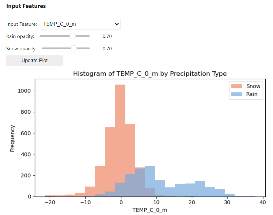
We'll start by visualizing the graphical distribution of values as histograms. In the plotting widget below, you can choose to view all data, or visualize the differences in distribution by precipitation type.

Instructions

Execute the two cells below.

In the Input Features widget, select an input feature from the dropdown menu then select Update Plot to view the data. Repeat to view any and all input features of interest.

Optionally, adjust the opacity of the rain and snow classes for better viewing. After adjusting the sliders, select Update Plot.

from applications_tech import HistogramWidget

widget = HistogramWidget(df)
widget.display()

We can also supplement these graphical representations of spread with a summary statistics table. Examine the statistics to locate any unusual values, or those that do not seem to be physically plausible.

Instructions

Execute the cell below to generate a summary statistics table of the input features.

Use the left-right scroll bar to view all columns.

The table includes the following statistics.

label	definition
count	number of records
mean	arithmetic mean
std	standard deviation
min	minimum value
25%, 50%, 75%	25th, 50th, and 75th percentile of the distribution, respectively
max	maximum value

df.describe()

	TEMP_C_0_m	TEMP_C_1000_m	TEMP_C_5000_m	T_DEWPOINT_C_0_m	T_DEWPOINT_C_1000_m	T_DEWPOINT_C_5000_m	UGRD_m/s_0_m	UGRD_m/s_1000_m	UGRD_m/s_5000_m	VGRD_m/s_0_m	VGRD_m/s_1000_m	VGRD_m/s_5000_m	PRES_Pa_0_m	PRES_Pa_1000_m	PRES_Pa_5000_m
count	5000.000000	5000.000000	5000.000000	5000.000000	5000.000000	5000.000000	5000.000000	5000.000000	5000.000000	5000.000000	5000.000000	5000.000000	5000.000000	5000.000000	5000.000000
mean	3.632016	-0.746313	-19.925755	1.130736	-2.172693	-27.131464	0.445190	3.266774	17.300987	-0.873734	1.544326	7.710204	97618.754410	862.006982	514.001548
std	8.372067	8.707363	8.836249	8.183560	8.601649	12.731960	3.805889	9.232793	12.732507	3.654125	9.584163	13.679516	4327.897516	38.665003	27.168435
min	-21.328827	-26.929945	-50.282283	-25.157257	-46.479145	-75.300519	-13.402076	-36.590512	-27.972064	-13.447640	-40.431958	-50.363994	66256.414062	581.237407	329.045904
25%	-1.437222	-6.585131	-26.066483	-3.862354	-7.727319	-35.558317	-2.092202	-2.399888	8.198301	-3.312952	-4.517914	-0.581500	97056.430915	856.920760	505.621304
50%	1.536438	-2.625801	-19.572960	-0.336419	-3.439562	-25.175794	0.106456	3.612947	17.815394	-0.772208	1.322942	7.652779	98584.171875	870.712713	517.785398
75%	6.498490	3.419899	-13.744804	4.214766	2.339916	-17.693843	2.994793	9.578508	26.319220	1.518725	7.466151	16.348368	99859.810250	882.060269	529.149799
max	37.702423	28.435911	3.553120	26.039459	21.696786	2.395806	20.642594	32.714230	62.565679	11.930449	42.105092	64.503670	103254.549774	913.848392	563.221716

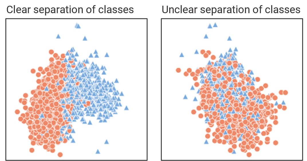
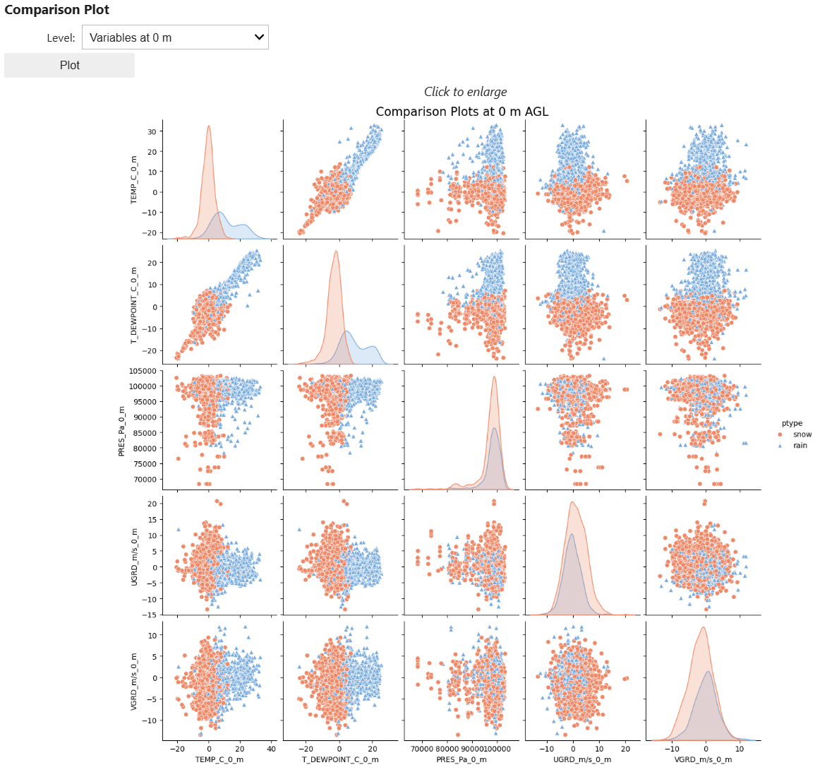
Next we'll compare the input features more directly by comparing all records in a grid of plots. In these comparison grids, the scatter plots display the input features a given time. For example, the temperature at 0 m on the x-axis and the dewpoint at 0 m on the y-axis. The scatter plot markers denote the precipitation type, blue triangles for rain and red circles for snow. Scatter plots that show distinct clustering of precipitation types demonstrate that the input variables may be better predictors of rain versus snow. Where rain and snow markers are uniformly distributed, the input features show reduced skill in differentiating rain and snow.

The comparison plot grid displays histograms where the x- and y-axes are the same station. These are the same histograms that you plotted previously, displaying the distribution of all records by precipitation type.

Instructions

Execute the cell below to generate the comparison plot.

from applications_tech import display_correlation_plot_dashboard

display_correlation_plot_dashboard()

Exercise 2b

Open your Machine Learning Model Handbook to Exercise 2b. Then describe your exploratory data analysis of any target and input features of note. Include the following:

• How many rain and snow records are in the dataset?
• Do the distributions of values make sense for the physical world?
• Are there any unexpected values?
• Which input features may be the strongest predictors of rain vs snow?
• Include any important plots to illustrate your conclusions. Limit yourself to 5 plots.
  To copy a plot image, hold shift, right click on the image, then select Copy.

Part 2c: Create a data splitting strategy

Next we create a data splitting strategy. Data splitting refers to the process of dividing data into three groups: training, validation, and testing. Each of these groups represent a part of the iterative process for machine learning model development.

• Training data is the largest subset, usually around 60-80% of the total data, and is used to initially train the model.
• Validation data is roughly 10-20% of the total data, and is used to validate the effectiveness of the training process.
• Testing data is also roughly 10-20% of the total data, and is used to test the final refined model before using it on new, unseen data.

Each group should be separate to ensure no single group will bias the model. Sam and the team used the following percentages in their original model:

Group	Percent of total data
Training	75%
Validation	15%
Testing	10%

Instructions

Execute the cell below.

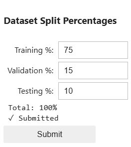
In the Dataset Split Percentages widget, input the percentages Sam used in their original model (above).

Select Submit after making your selection.

from applications_tech import create_percentage_widget

widget, get_values = create_percentage_widget()

Instructions

Execute the three cells below to execute the functions to split the data according to the percentages you submitted above.

decimals = get_values()
training = decimals['training']
validation = decimals['validation']
testing = decimals['testing']

from applications_tech import train_val_test_split

X_train, y_train, X_val, y_val, X_test, y_test = train_val_test_split(df, 
                                                                      y_col='ptype',
                                                                      train_size=training,
                                                                      val_size=validation,
                                                                      test_size=testing)

---

Part 3: Model Development

Next begins the iterative process of creating, evaluating, and refining the machine learning model. You will start by recreating Sam's original model and critically evaluating its performance. Then, you will refine the model based on your own choices, keeping track of your trials in your Machine Learning Model Handbook.

Click to enlarge

Part 3a: Choose Algorithm

When selecting an algorithm, we want to choose an algorithm that is appropriate for the data and isn't prone to overfitting. Sam's team considered the following two algorithms: LogisticRegression (Linear) and Random Forest. Despite its name, the LogisticRegression (Linear) algorithm is used for classification tasks. This is because at its core, this algorithm predicts the likelihood of a record being rain or snow. It then returns the most likely classification. You can read more about each algorithm in the information below.

About the Algorithms

LogisticRegression (Linear)

• Works well for simple problems: If your data is not too complex, it often gives good results.
• Fast & efficient: It trains quickly, even on large datasets.Fast & efficient: It trains quickly, even on large datasets.
• Less likely to overfit: It doesn’t easily memorize the training data.
• Struggles with complex patterns: If the decision boundary isn’t a straight line, linear regression may not work well.
• Sensitive to outliers: A few extreme values can heavily influence the model, making it less reliable.

Random Forest

• Handles complex data well: Random Forest can model complex, nonlinear patterns in the data.
• Not sensitive to outliers: A few extreme values won't throw off the model like they might in a linear algorithm.
• Good accuracy: It's often more accurate than simpler models.
• Moderate risk of overfitting: Certain situations may cause the algorithm to create a decision boundary that is too complex, or overfits to the training data.
• Slower and more computationally expensive: For large datasets, this algorithm takes much more time and computational power compared to the linear algorithm.

Sam and the team chose the LogisticRegression (Linear) algorithm to train their original model. While you will initially use this algorithm to recreate the original model, you will have an opportunity later to test other options.

Instructions

Execute the two cells below.

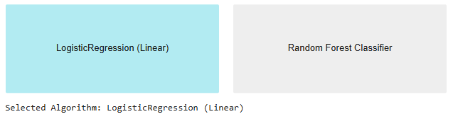
After executing algorithm_selection(), select LogisticRegression (Linear) to match Sam's choice.

You will learn more about both algorithms in a later step

from applications_tech import algorithm_selection

selected_algo = algorithm_selection()

Part 3b: Choose input features

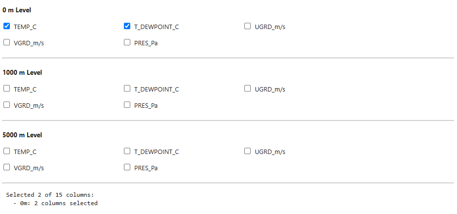
To recreate Sam's model, you'll use the same input features they used to create their original model. The features they chose are in the table below.

Sam's input features
TEMP_C_0_m
T_DEWPOINT_C_0_m

Instructions

Execute the two cells below.

After executing create_column_filter_widget(), select the input features used in Sam's model.

from applications_tech import create_column_filter_widget

widget, get_selected_columns = create_column_filter_widget()
display(widget)

Instructions

Execute the cell below to filter out any features that will not be used as input to the machine learning model.

X_train_filtered = X_train[get_selected_columns()]
X_val_filtered = X_val[get_selected_columns()]
X_test_filtered = X_test[get_selected_columns()]

Part 3c: Train the Algorithm

The training process is what transforms the machine learning algorithm into a supervised machine learning model. You will now train the algorithm to recreate Sam's model.

Instructions

Execute the two cells below.

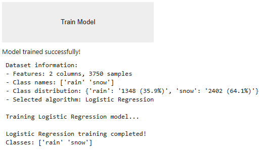
After executing train_button(), select the Train Algorithm button to initiate the training process. A progress printout will display below the button while the process runs.

from applications_tech import train_button

model_choice = selected_algo()
trained_model = train_button(model_choice, X_train_filtered, y_train)

Part 3d: Validate the Model

The validation step uses the separate validation dataset to evaluate how well the training process performed. The newly trained model takes the environmental variable input features from the validation dataset and outputs a rain or snow classification prediction. We can then take the predictions the model made and compare them to the known true classifications. By using a separate validation dataset to evaluate performance, we get a better sense of how well the model can generalize to new inputs.

Sam's team calculated the model's accuracy to determine how well the model performed, which you will also do in this step. Accuracy is defined as $$ \frac{\text{correct predictions}}{\text{total predictions}} $$

Recall that Sam's model returned an 88% accuracy initially.

Instructions

Execute the two cells below. The model accuracy should be close to the 88% that Sam and the team originally found.

# Get the model
model = trained_model()

y_pred = model.predict(X_val_filtered)

from sklearn.metrics import accuracy_score, precision_recall_fscore_support, confusion_matrix

# Get accuracy metric
accuracy = (accuracy_score(y_val, y_pred))*100
print(f"Original Model Accuracy (validation dataset): {accuracy:.2f}%")

Original Model Accuracy (validation dataset): 87.47%

Why does the model not produce 88% accuracy each time?

As discussed in the previous module, machine learning algorithms will generate and test multiple different decision boundaries each time the training process is run. The boundaries they generate are unlikely to be the same each time because of the nature of algorithms. This is a demonstration of machine learning being an approximator and not an exact solution, like an algebraic formula.

Other evaluation metrics

While accuracy gives a broad view of how well the model performs, we don't know the specifics. Does the model struggle to classify just rain, just snow, or both? You will calculate additional statistics for Sam and the team to provide additional insight into the model's performance.

Confusion matrix

A confusion matrix is a visual representation of all the predictions the model made. In this two-class model, there can be four kinds of outputs:

• Predicted rain, and the true observation (target feature) was rain
• Predicted rain, but the true observation was snow
• Predicted snow, but the true observation was rain
• Predicted snow, and the true observation was snow

The confusion matrix shows the number of each of these types outputs in a grid, so we can visualize the predictions that the model generated.

Instructions

Execute the two cells below to generate the confusion matrix.

from applications_tech import plot_confusion_matrix

fig = plot_confusion_matrix(model.classes_, y_true=y_val, y_pred=y_pred, 
                           title='Original Model Confusion Matrix')
plt.show()

The values in the confusion matrix can then be used to quantify additional model evaluation metrics. These metrics help answer specific questions about how well the model performs.

Precision

Precision is a measure of correct predictions for each class. It answers the question "When the model predicts rain (or snow), how often is it correct?" We calculate the precision of the rain class by

$$ \frac{\text{correct rain predictions}}{\text{correct rain predictions + incorrect rain predictions}} $$

For example, a rain precision value of 0.65 would tell us that of the times that the model predicted rain, it was correct only 65% of the time. A high-performing model would have a precision value close to 1.

Recall

Recall is a measure of how well the model predicts the correct classification for each class. It answers the question "Out of all actual rain (or snow) cases, how many did the model correctly predict?" We calculate it as

$$ \frac{\text{correct rain predictions}}{\text{total actual rain cases}} $$

For example, a rain recall value of .81 would tell us that of all of the true rain cases in the dataset, the model correctly predicted rain in 81% of them. A high-performing model would have a recall value close to 1.

Comparing Precision and Recall

These metrics may seem very similar, but they differ in the types of questions they answer. The table below demonstrates the differences in high and low precision and recall for one class (rain).

	High Precision, Low Recall	High Recall, Low Precision
What happens?	The model is very careful when predicting rain, but it misses a lot of actual rain cases.	The model catches almost all rain cases, but it also makes mistakes, calling snow "rain" a lot.
Example	Predicts "rain" only when very sure, leading to fewer false alarms but missing real rain.	Predicts "rain" too often, ensuring real rain isn’t missed but causing more false alarms.

Instructions

Execute the cell below to generate the original model's precision and recall for each class.

precision, recall, _, _ = precision_recall_fscore_support(y_val, y_pred, average=None, labels=['rain', 'snow'])

print("Original Model Validation Metrics")
print(f"Rain Precision: {precision[0]:.3f}")
print(f"Snow Precision: {precision[1]:.3f}")
print(f"Rain Recall: {recall[0]:.3f}")
print(f"Snow Recall: {recall[1]:.3f}")

Original Model Validation Metrics
Rain Precision: 0.896
Snow Precision: 0.866
Rain Recall: 0.736
Snow Recall: 0.952

Part 3e: Evaluate and Refine the Model

Examine the results of the original model validation and determine what each metric means. Review the descriptions of the evaluation metrics, then complete the next exercise.

Exercise 3e

Open your Machine Learning Model Handbook to Exercise 3e.

Paste the validation evaluation metrics in the designated box.

Then describe the results of the original model validation. Include the following:

• How well does the model predict rain? Support your description with the evaluation metrics.
• How well does the model predict snow? Support your description with the evaluation metrics.
• How do you interpret these statistics in the context of the physical world?
• What changes will you make to try to improve these statistics in the next iteration?

Part 3f: Iterative Refinement Trials

Now that you have recreated Sam's original model, it's now your turn to apply the information you have to refine it. Next, you'll create new trials to improve the evaluation metrics from the validation phase. You may complete as many trials as you like until you are satisfied with the evaluation metrics, or they no longer improve with new trials.

Instructions

Execute the code cells below, selecting your desired model configurations after executing each cell.

After each new trial, you will copy the validation metrics in your handbook document. See Exercise 3f.

You may complete as many trials in this section (3f) as you like until you are satisfied with the evaluation metrics, or they no longer improve with new trials.

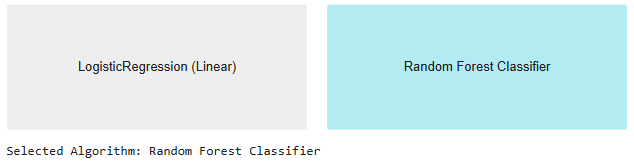
New trial: Choose algorithm

In the new trials, you have the option of choosing a new algorithm to train. Review the information about each of the algorithms in section 3a, then make your selection. Remember, you can run as many trials as you'd like.

selected_algo2 = algorithm_selection()

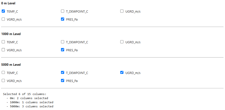
New trial: Choose input features

Sam used environmental variables at the surface level to train the algorithm. As you've seen from the Data Handling phase, the dataset also includes environmental variables at other levels that may provide additional predictive skill. Choose as many input features as you like, but recall that more data doesn't always produce a better model. Recall the comparison plots from section 2b and be strategic in your selections.

widget, get_selected_columns2 = create_column_filter_widget()
display(widget)

X_train_filtered = X_train[get_selected_columns2()]
X_val_filtered = X_val[get_selected_columns2()]
X_test_filtered = X_test[get_selected_columns2()]

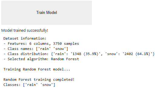
New trial: Train algorithm

Now, train the algorithm with your selected input features

model_choice = selected_algo2()
trained_model2 = train_button(model_choice, X_train_filtered, y_train)

New trial: Validate model

Generate the corresponding confusion matrix and validation metrics.

from applications_tech import classification_model_eval

model2 = trained_model2()
validation_metrics = classification_model_eval(model2, X_val_filtered, y_val, title='Validation')

Validation Metrics
Model Type: RandomForestClassifier
Input Features: TEMP_C_0_m, VGRD_m/s_0_m, T_DEWPOINT_C_1000_m, TEMP_C_5000_m, T_DEWPOINT_C_5000_m
 
Accuracy: 90.53%
Rain Precision: 0.927
Snow Precision: 0.896
Rain Recall: 0.799
Snow Recall: 0.965

Exercise 3f

• In your Machine Learning Model Handbook Exercise 3f, paste the full output of each of your validation trials, one per box.
• You may complete as many trials as you like until you are satisfied with the evaluation metrics, or they no longer improve with new trials. When complete, move on to the next part below.

Part 3g: Test Model

Important

For testing, your model needs to be in a state with your desired algorithm and input features. If you haven't already, go back and run through the cells in Part 3f with your final choices one last time. This ensures that your final testing process will be executed with your desired choices.

At this point, you have a trained model with validation metrics you are satisfied with. Next, it's time to test the model on brand new data: the testing dataset. The testing process mimics how the model would be used in a real-world process in a final, unbiased way.

Testing looks very similar to validation. You will again review the confusion matrix, accuracy, precision, and recall, but this time the predictions are made with the testing datset.

Instructions

Execute the cell below.

After executing classification_model_eval(), your model's testing metrics will appear below as a printout.

test_metrics = classification_model_eval(model2, X_test_filtered, y_test, title='Testing')

Testing Metrics
Model Type: RandomForestClassifier
Input Features: TEMP_C_0_m, VGRD_m/s_0_m, T_DEWPOINT_C_1000_m, TEMP_C_5000_m, T_DEWPOINT_C_5000_m
 
Accuracy: 90.20%
Rain Precision: 0.918
Snow Precision: 0.894
Rain Recall: 0.802
Snow Recall: 0.959

Part 3h: Evaluate and Justify

Your final decision

Given all your evaluation, it's time to make a final recommendation to Sam and the team on whether you believe this model provides sufficient skill for the needs of the situation. Go back and review the problem statement. Does this model deliver the results needed?

Exercise 3h

Open your Machine Learning Model Handbook to Exercise 3h.

Paste your testing evaluation metrics in the designated box.

Then make a final decision on whether this model delivers on the results needed with supporting justification. Include the following:

• Which precipitation class(es) had the best evaluation metrics? List some physical scientific reasons why this may be the case.
• Is this model ready for use in the real world? Why or Why not?
• What other possible changes could further improve this model?

---

Conclusion

No matter your final decision, the most important aspect is your ability to justify it using data and a robust evaluation. In real-world applications, decision makers rely on this type of analysis to assess risk, costs, and benefits. Rarely is there a single correct answer. What matters is the reasoning behind your choices and how well they align with the environmental context. As you continue learning and exploring new machine learning techniques, remember that each model you build is an opportunity to deepen your understanding. With each step, you gain the expertise to make informed, justifiable decisions that contribute to meaningful scientific and real-world advancements.

---

Acknowledgements

This work was supported by NSF Unidata under award #2319979 from the US National Science Foundation. Any opinions, findings, and conclusions or recommendations expressed in this material are those of the author(s) and do not necessarily reflect the views of the National Science Foundation.

We thank the NOAA National Severe Storms Laboratory for contributing mPing data to this project. We also thank NCAR MILES for data processing and support.